How to Create Excel Formulas from Basic to Advanced

You’ve opened a workbook that looks simple enough, but the totals don’t match, a copied formula points at the wrong column, and someone has left a note saying, “Just fix the IF.” You can create Excel formulas that calculate correctly, but reliable spreadsheet work requires more than remembering syntax. You also need to understand references, test edge cases, trace dependencies, and verify any formula generated by another person or by AI.

Table of Contents

• What You Will Be Able to Build With Excel Formulas
  • A practical progression
• Foundations Every Formula Relies On
  • The four operator groups
  • Parentheses prevent plausible mistakes
• Core Functions That Handle Most Real Work
• Nesting and Array Formulas Explained
  • Read the layers before shortening the workbook
• Debugging Formulas When Something Goes Wrong
  • Read the error as a diagnosis
  • Trace the calculation instead of guessing
• Auditing and Trusting Your Formulas at Scale
  • Test the cases that make formulas lie
  • Protect the finished logic
• Your Formula Creation Checklist

What You Will Be Able to Build With Excel Formulas

If you already use Excel, you may be entering values manually, copying formulas from colleagues, or changing cell references until the result looks right. That approach works for a quick calculation, but it becomes fragile when the workbook grows or someone else needs to maintain it. Formulas are reusable building blocks, not one-off answers.

Excel has been part of business work for decades. Microsoft first launched Excel on the Macintosh in September 1985 and marked 40 years of Excel in 2025. Microsoft’s workbook statistics feature now counts formulas at worksheet and workbook levels, which reflects how central formulas have become to everyday spreadsheet files. Research across a large spreadsheet corpus also found IF appearing 30,798,987 times before deduplication, making it a useful starting point for learning practical spreadsheet logic. Microsoft’s history of Excel and the spreadsheet datasets and benchmarks research both show why formula literacy matters.

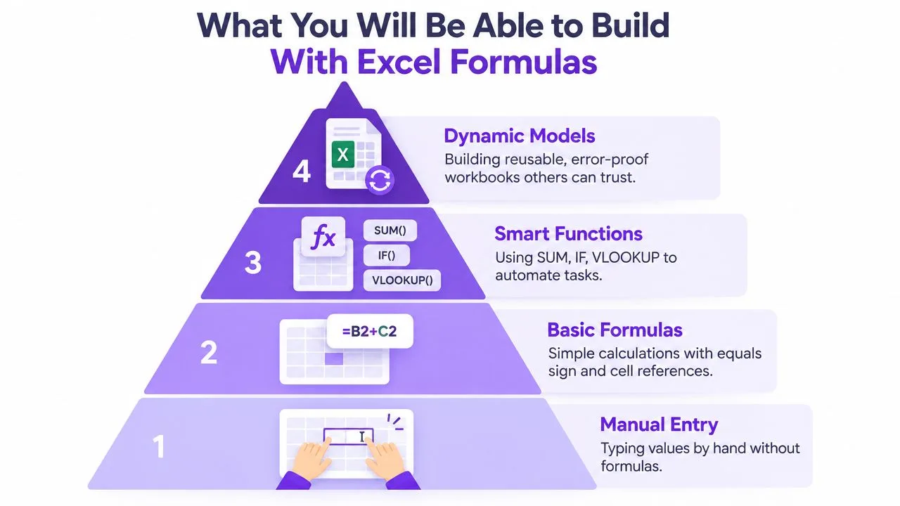
A practical progression

Start with a column total such as =SUM(B2:B20). Then add conditions, for example, summing revenue only for a selected region with SUMIFS. From there, you can build a nested IF that classifies records, or use XLOOKUP to bring prices and categories into a transaction table.

The final step is a small dynamic dashboard. A dropdown in B1 can control a formula that filters sales, updates a summary, and feeds a chart. The examples here use small ranges so you can see the logic clearly, but the same habits apply to operational workbooks with multiple sheets and inconsistent source data.

By the end, you should be comfortable with:

• Basic calculations: Totals, differences, percentages, and date arithmetic.
• Conditional logic: Nested IF statements and criteria-based summaries.
• Lookups: VLOOKUP for older files and XLOOKUP for newer designs.
• Dynamic results: FILTER, SORT, and UNIQUE formulas that spill into neighboring cells.
• Quality control: A repeatable process for checking references, testing unusual inputs, and tracing failures.

Foundations Every Formula Relies On

Every Excel formula starts with an equals sign. It tells Excel to interpret what follows as an expression rather than ordinary text. For example, =B2*C2 multiplies the quantity in B2 by the unit price in C2.

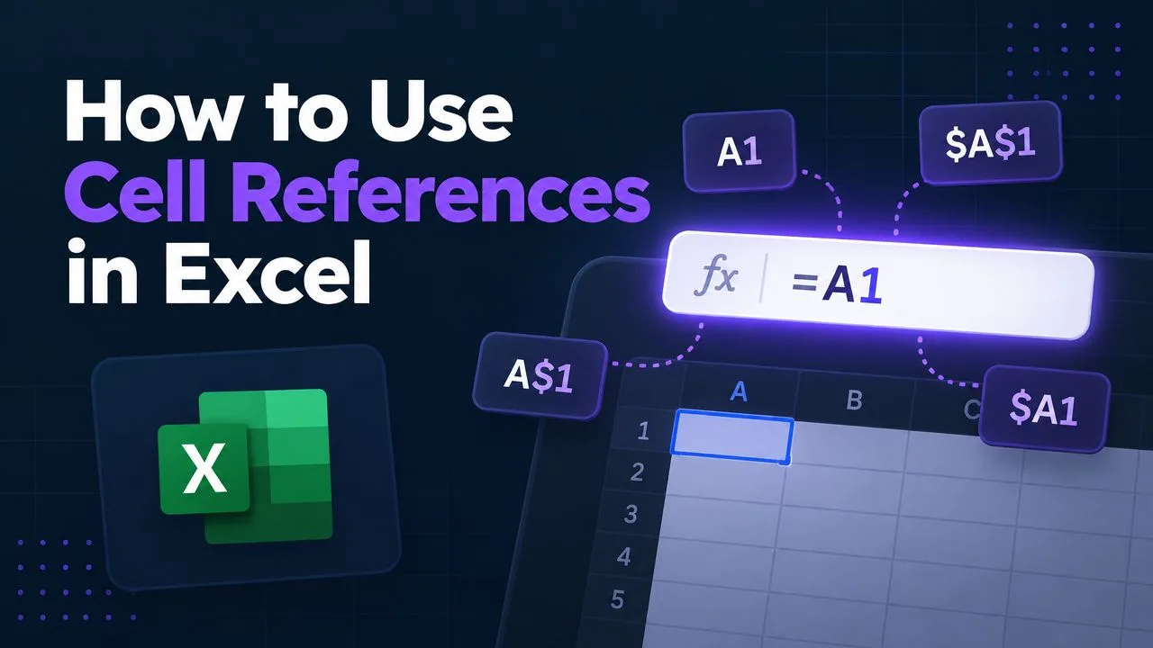
Cell references determine how a formula behaves when you copy it. A relative reference such as A1 changes when moved, so a formula in row two can become a row-three formula when filled down. An absolute reference such as $A$1 stays fixed. Mixed references lock only one dimension: A$1 keeps the row fixed, while $A1 keeps the column fixed.

The four operator groups

Arithmetic operators perform calculations:

• Arithmetic: +, -, *, /, and ^. =B2*C2 multiplies two cells, while =B2^2 squares a value.
• Comparison: =, <>, <, >, <=, and >=. =B2>100 returns TRUE when the value exceeds the threshold.
• Text concatenation: & joins text. =A1&A2 combines the contents of two cells, while =A1&" "&A2 inserts a space.
• Reference operators: : creates a range, as in A1:A10; a comma combines references, and a space returns an intersection where the referenced ranges overlap.

The difference between relative and absolute references becomes obvious with a tax example. If the tax rate is stored in F1, use =B2*$F$1 before filling the formula down. Without the dollar signs, F1 would move to F2, F3, and so on, producing incorrect results unless every row contains the intended rate.

Parentheses prevent plausible mistakes

Excel follows an order of operations. Multiplication and division are handled before addition and subtraction, so =A1+B1*C1 isn’t the same as =(A1+B1)*C1. Use parentheses whenever the business rule matters more than the default order.

Practical rule: If a formula represents a sentence such as “add the discount, then multiply by the quantity,” write the parentheses so another person can read that rule directly.

Core Functions That Handle Most Real Work

A small group of functions covers many recurring tasks. The syntax matters, but the choice of range and treatment of missing data matter just as much.

IF branches based on a condition. Use `=IF(C2

Nesting and Array Formulas Explained

Nesting places one function inside another, so the result from an inner calculation becomes an input for an outer rule. For example, =IF(SUM(B2:B5)>1000,"Review","Clear") totals the values first, then checks whether the total passes the threshold. Read formulas from the inside out, just as you would verify each stage of a spreadsheet calculation.

Suppose B2 contains the customer type, C2 the unit price, and D2 the quantity. A valid compact pricing formula is =ROUND(IF(B2="Member",C2*D2*0.9,C2*D2),2). It calculates the line value, applies the member discount when appropriate, and rounds the result. Eligibility rules covering many rows belong in a helper column or a range-based SUMIFS, where the sum range and criteria ranges are explicit and can be checked separately.

Read the layers before shortening the workbook

Short formulas are not automatically easier to maintain. If several rules are nested together, a reviewer may struggle to identify which condition produced an unexpected amount. Once a formula grows beyond a few logical layers, helper columns can make each step easier to test, audit, and hand over.

Step	Function Layer	Purpose	Example Output
1	SUMIFS	Select matching sales	Eligible sales total
2	IF	Apply a business rule	Discounted or standard value
3	ROUND	Control displayed precision	Final amount

Dynamic array formulas return multiple results from one cell. =FILTER(A2:D100,D2:D100="Open") returns open records and spills them into nearby cells. =SORT(A2:D100,3,-1) sorts that returned range by its third column, while =UNIQUE(B2:B100) creates a distinct list for a dropdown or summary.

Check the intended spill area before judging the formula. A value blocking one destination cell can produce #SPILL!, even when the filtering or sorting logic is correct. Clear the obstruction, then validate the returned rows against the source data.

Older workbooks may use legacy array formulas entered with Ctrl+Shift+Enter. Excel shows curly braces around them in the formula bar, although you do not type those braces. Keep them intact when maintaining older designs, and prefer dynamic arrays for new work when the workbook supports them.

For drafting help, a Google Sheets formula generator can suggest syntax. Review its ranges, conditions, and sample output against the actual workbook before using the formula.

Debugging Formulas When Something Goes Wrong

A wrong result doesn’t always produce an obvious error. Microsoft’s formula guidance calls out common failures such as omitting the leading equals sign, mismatching parentheses, misunderstanding operator precedence, and treating a cell as blank when it contains hidden content. Microsoft Press documents 11 Excel error types, including #REF!, #VALUE!, #N/A, #SPILL!, and #CALC!, so the visible message is an important clue.

Start with Excel’s background error checking and the Error Checking tool. Then inspect the formula’s relationships. Microsoft’s formula error detection guidance recommends using Error Checking, Trace Precedents, and Evaluate Formula as part of a structured workflow.

Read the error as a diagnosis

• #DIV/0! means a calculation divides by zero or an empty denominator.
• #N/A commonly means a lookup found no match.
• #NAME? indicates unrecognized text, often a misspelled function or missing quotation marks.
• #NULL! points to an invalid range intersection.
• #NUM! signals an invalid numeric operation.
• #REF! means a reference was deleted or is no longer valid.
• #VALUE! usually indicates an incompatible data type.
• #GETTING_DATA appears while Excel is retrieving information.
• #SPILL! means the dynamic result can’t occupy its output range.
• #CALC! indicates a calculation problem, often involving an unsupported array result.
• #UNKNOWN! indicates Excel can’t identify the requested calculation or content.

Select the problem cell and press F2 to enter edit mode. Check each range, parenthesis, and argument. If the formula bar becomes difficult to use, Ctrl+Backspace resets the editing view. You can also highlight a subexpression in the formula bar and press F9 to evaluate that portion. Press Esc afterward so you don’t accidentally replace the formula with the displayed value.

Trace the calculation instead of guessing

Trace Precedents draws arrows from input cells into the selected formula. Trace Dependents shows where the result flows, which is especially useful before changing a summary cell. Evaluate Formula walks through a nested expression one piece at a time, helping you identify the exact term that changes from a sensible value to an error.

The sequence is simple: check the error indicator, trace the inputs, evaluate the expression, correct the smallest broken piece, and recalculate. Don’t begin by rewriting the entire formula. That often removes useful clues.

Watch the debugging tools in action before applying them to a live workbook.

Auditing and Trusting Your Formulas at Scale

Treat an operational formula like code that someone else will inherit. Independent spreadsheet-auditing research found errors in 0.9% to 1.8% of formula cells across 50 operational spreadsheets, depending on how the researchers defined an error. The wide variation between workbooks is the important lesson, so the auditing methodology supports systematic workbook-level review rather than casual spot-checking.

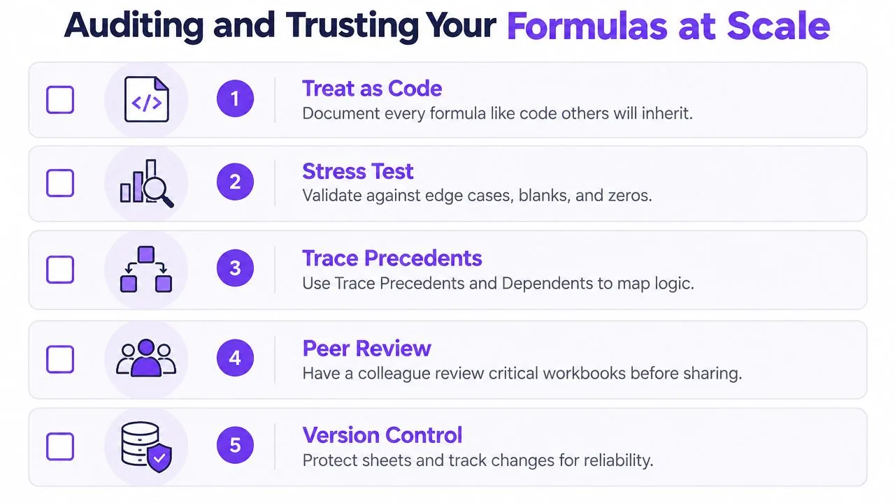
Test the cases that make formulas lie

Before sharing a report, deliberately test blank cells, text inside numeric columns, negative values, zero-length strings, and missing lookup keys. Compare each result with a known manual calculation. A formula that returns a plausible number can still apply the wrong condition or reference the wrong period.

Use Name Manager to give important ranges meaningful names such as ApprovedSales or TaxRate. A formula like =SUM(ApprovedSales) communicates intent more clearly than a long address, provided the named range remains accurately maintained.

The Watch Window helps you monitor critical cells while editing other sheets. The Inquire add-in can help compare workbook versions and inspect relationships, including references that aren’t obvious during normal navigation. Availability can depend on your Excel edition and organizational setup, so confirm that the tool is enabled before designing a process around it.

Protect the finished logic

After review, use sheet protection to prevent accidental edits to formulas. Hide sensitive formula entries where appropriate, but remember that protection is a control, not a substitute for documentation or version management.

Consider a monthly revenue report where a column insertion leaves a formula pointing at the wrong field. The result may still look like a valid number. A named range, a precedent trace, a comparison with the prior version, and a test row with a known expected result would have exposed the problem during construction instead of after the executive meeting.

Your Formula Creation Checklist

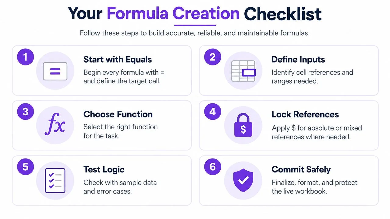
Use this checklist every time you add a formula to a live workbook. It turns formula creation into a small review process rather than a guessing exercise.

1. Start with the equals sign: Select the intended target cell and begin with =. This prevents Excel from storing the expression as text.
2. Define the inputs: Write down the cells, ranges, criteria, and expected output type. Decide whether the result should be numeric, text, a date, or a spilled range.
3. Choose the function: Start in a scratch cell. Pick SUM, IF, SUMIFS, XLOOKUP, TEXT, DATE, or another function that matches the rule.
4. Lock references: Add $ to rates, lookup tables, and fixed criteria cells before copying. Check mixed references such as A$1 and $A1 deliberately.
5. Test the logic: Compare the formula with a known value, then test blanks, text, zeros, negative values, and missing matches. Use Error Checking and Evaluate Formula when the result is unclear.
6. Commit safely: Add a brief cell comment or nearby note describing the intent, format the output, and protect the finished formula when other users shouldn’t edit it.

These steps target the failures that cause the most trouble: unanchored ranges that shift during copying, incorrect argument counts, and silent wrong results that surface months later. If you use AI to draft a formula, apply the same checks. Microsoft’s Excel Copilot guidance tells users to review the suggested formula and confirm that its references and logic match the dataset before applying it. For Google Sheets workflows, using AI in Google Sheets can help with drafting and analysis, but verification remains your responsibility.

---

GPT Workspace works inside Google Workspace applications and can help draft Sheets formulas, analyze selected ranges, clean data, and turn plain-language requests into spreadsheet logic. Visit GPT Workspace to test a workflow where formula generation and spreadsheet review happen in the same workspace, then apply the validation checklist before publishing your next report.