Google Sheets Lookup Functions Explained and Compared

You’re staring at a google sheets lookup formula that looked fine in testing, then a new import lands and half the rows come back wrong. The sheet still calculates, the dashboard still refreshes, but the values don’t line up with reality, which is exactly the kind of bug that wastes an afternoon because it doesn’t always throw an obvious error.

Lookup functions in Google Sheets are useful because they turn messy tables into usable records, and Google’s own function catalog makes that clear with LOOKUP, MATCH, and VLOOKUP sitting in the official lookup family, plus the newer XLOOKUP option for exact-match retrieval Google Sheets function list. The problem is that the formulas people memorize are not the same as the formulas that survive production data, duplicate keys, hidden spaces, and imported CSV weirdness.

Practical rule: if a lookup worked yesterday and fails today, assume the data changed before you assume the formula is wrong.

Table of Contents

• Why Lookup Formulas Break in Real Spreadsheets
  • The usual failure pattern
  • What to check first
• VLOOKUP Syntax and Practical Examples
  • Exact match versus approximate match
  • The structural limit that trips people up
• XLOOKUP as the Modern Default for Exact Match Retrieval
  • Why the syntax matters
  • Exact match and missing values
• INDEX and MATCH for Flexible Two-Part Lookups
  • How the two functions split the job
  • Multi-criteria lookups
• HLOOKUP and Legacy Lookup Functions
  • Where MATCH stands on its own
  • When these still earn a spot
• Choosing the Right Lookup Function for Your Data
• Troubleshooting Common Lookup Formula Errors
  • The issues I check most often
• Generating and Debugging Lookup Formulas with GPT Workspace
  • A practical use pattern
• Quick Reference for All Google Sheets Lookup Functions

Why Lookup Formulas Break in Real Spreadsheets

A broken lookup usually starts with a sheet that looks clean to the eye and is anything but clean under the hood. A product ID is stored as text in one table and as a number in another. A vendor export adds a trailing space. Someone sorts part of a range and leaves the rest untouched. The formula still runs, but the match logic is now looking at the wrong thing.

That’s why google sheets lookup work is less about memorizing syntax and more about reading the data structure. Google’s legacy LOOKUP function is documented as working through a sorted row or column, while MATCH returns the relative position of a matching item, which tells you these tools were built with specific data assumptions in mind Google Sheets function list. In practice, those assumptions are exactly where production sheets tend to fail.

The usual failure pattern

A formula gets built against a small clean sample. Then the sheet arrives with duplicate keys, imported values, and mixed formatting. The result is either a visible error like #N/A or a much worse silent mismatch that returns the wrong row without warning.

How to merge cells in Google Sheets is not the right fix here, because merged layout issues often hide the structural problem rather than solving it.

What to check first

• Key formatting: Confirm the lookup key is the same type on both sides, especially for IDs and ZIP-like fields.
• Whitespace: Trim leading and trailing spaces before blaming the formula.
• Duplicates: Decide whether the first match is acceptable, because many lookup functions stop there.
• Sort order: If you rely on approximate matching, verify the range is sorted.

The cleanest lookup formula is still only as reliable as the data it points at.

VLOOKUP Syntax and Practical Examples

VLOOKUP remains the function many users reach for first because its structure is familiar and easy to explain. Google’s help page defines the syntax as =VLOOKUP(search_key, range, index, [is_sorted]), and that shape is still the backbone of a lot of spreadsheet retrieval work Google Sheets VLOOKUP help. It searches down the first column of a range and returns a value from another column in the same row.

Suppose a catalog sheet stores Product ID in column A and Price in column C. A VLOOKUP can take the ID from your order sheet, scan column A, and return the matching price from column C. That part is straightforward, which is why the function shows up in so many operational workbooks.

Exact match versus approximate match

The danger is the is_sorted argument. If you want a precise result, use FALSE. If you omit it or use TRUE, VLOOKUP treats the search differently and expects sorted data, which can produce wrong answers when the range isn’t organized the way the function expects Google Sheets VLOOKUP help.

If the data isn’t deliberately sorted for approximation, treat TRUE as a liability, not a convenience.

The structural limit that trips people up

VLOOKUP can only search the leftmost column of the selected range and return values to the right. That means the lookup column has to sit at the start of the range, or you have to rearrange the table. In production sheets, that usually means one of three things, moving columns, adding helper columns, or switching functions.

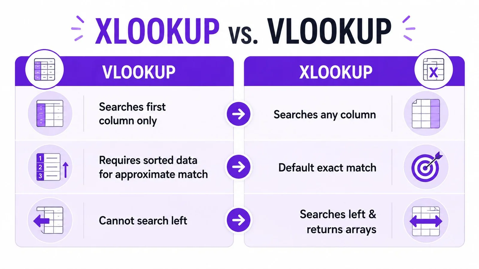
The cleanest VLOOKUP use case is still simple, vertical, left-to-right retrieval. Once the lookup column moves or the data stops being orderly, the formula starts working against you instead of for you.

XLOOKUP as the Modern Default for Exact Match Retrieval

XLOOKUP is the lookup function I reach for first on new sheets because it separates the lookup range from the result range. That single design change removes the left-to-right restriction that makes VLOOKUP awkward in real data models, and Google’s help page describes the function as returning values from a result range based on the matched position in a lookup range Google Sheets XLOOKUP help. In practice, that means the formula is easier to read and easier to maintain.

The other reason it matters is failure handling. Google notes that XLOOKUP’s default behavior returns the closest match only when an exact match isn’t found, which is why the missing_value argument matters if you want predictable output Google Sheets XLOOKUP help. In production sheets, silent fallback behavior is rarely what you want.

Why the syntax matters

With XLOOKUP, the lookup key can sit in one column, the return value in another, and the function doesn’t care whether the return column is left or right of the key. That flexibility removes a lot of helper columns and range reshuffling. It also makes cross-sheet retrieval easier to read when the source table is already structured well.

Exact match and missing values

For exact-match workflows, the safer pattern is to spell out the not-found result instead of letting the formula improvise. That’s especially important in operational dashboards, where a blank or explicit message is better than an accidental approximate result.

A good XLOOKUP formula is less about cleverness and more about control.

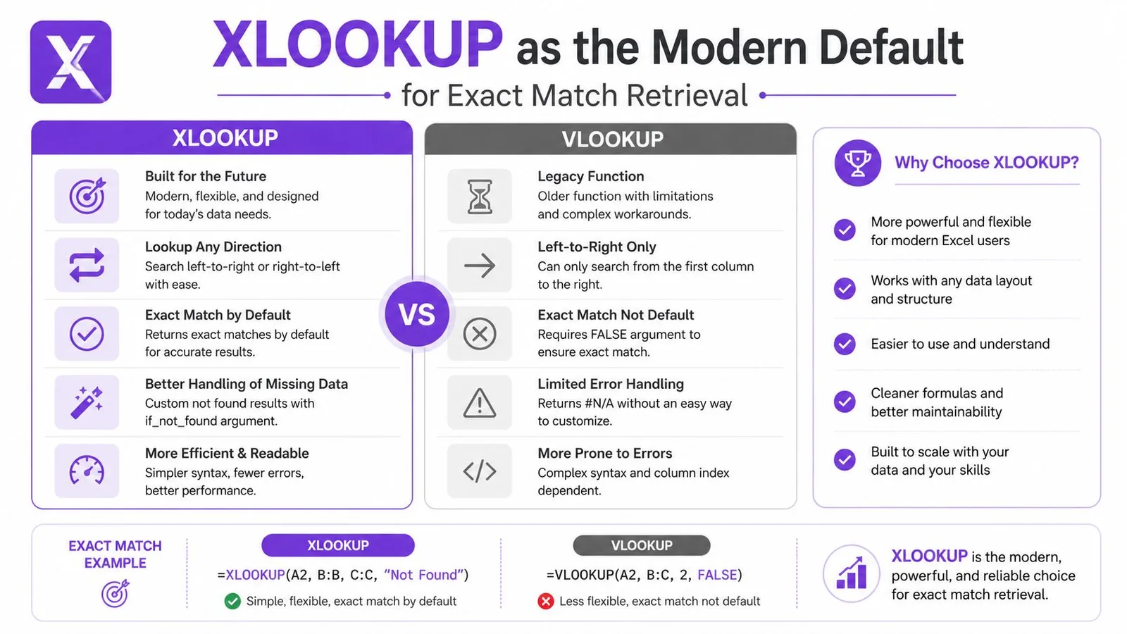
For teams working with imported tables, messy extracts, or columns that don’t sit neatly on the left edge, XLOOKUP is usually the cleaner default. VLOOKUP still has a place in older workbooks and in simple approximate-match models, but for exact retrieval, XLOOKUP is the function that causes fewer avoidable rewrites.

INDEX and MATCH for Flexible Two-Part Lookups

Before XLOOKUP was available, INDEX/MATCH was the standard escape hatch for VLOOKUP’s column restriction, and it still earns its place when a workbook already depends on it. Google’s function list categorizes MATCH as returning the relative position of an item that matches a specified value, which is exactly what makes the pair work so well Google Sheets function list. MATCH finds the row or column position, then INDEX returns the value from the corresponding position in another range.

How the two functions split the job

MATCH answers one question, where is the key. INDEX answers the other, what value lives at that position. That separation is useful when the lookup column is to the right of the return column, because you’re no longer forcing the key to be the first column in a range.

A simple way to think about it is this. VLOOKUP searches the table and returns a column. INDEX/MATCH searches one range and returns from another, which gives you more control over table design and fewer reasons to rearrange source data.

Multi-criteria lookups

INDEX/MATCH also shows up in multi-criteria setups where one key isn’t enough. In those cases, teams often combine conditions so the formula matches the right row only when all criteria line up. In Google Sheets, that pattern often needs careful array handling, because copying an Excel-style formula down column by column can break the logic or hide the intended spill behavior.

Useful habit: when an INDEX/MATCH formula gets hard to read, stop compressing it. Separate the position logic from the return logic and test each part on its own.

XLOOKUP is simpler for most new work, but INDEX/MATCH still matters in older files, compatibility-heavy environments, and models where the formula design already depends on its flexibility.

HLOOKUP and Legacy Lookup Functions

Google Sheets still includes lookup tools that make sense in narrow layouts, and HLOOKUP is the main one. Instead of searching down columns, it searches across rows, which is handy when your data is transposed or built like a pivot-style summary. If your categories run horizontally, HLOOKUP can be the direct answer instead of a forced rewrite.

The older LOOKUP function is more limited and more brittle. Google documents it as working through a sorted row or column and returning a corresponding value, which makes it useful only when the source data already fits that model Google Sheets function list. That sorted-data requirement is why LOOKUP is rarely the right default for modern imported tables.

Where MATCH stands on its own

MATCH is also useful by itself when you only need a position, not the final value. That’s common in formulas that build dynamic references or feed another function that needs the index number instead of the raw data. It’s a small function, but it gives the rest of the formula structure.

When these still earn a spot

• HLOOKUP: Use it when the table is naturally horizontal and you don’t want to transpose it.
• LOOKUP: Use it only when the data is already sorted and the simple legacy behavior fits.
• MATCH: Use it when position matters more than the returned value.

These are specialized tools, not universal defaults. They’re worth keeping in your toolkit, but they’re not where I’d start on a new sheet.

Choosing the Right Lookup Function for Your Data

The decision is usually simpler than the formula syntax makes it look. Start with the shape of the data, then ask whether you need an exact match, an approximate match, or support for duplicate handling. If the table is vertical and the key is on the left, you have more options. If the data is messy or imported, fewer of them are comfortable.

Function	Direction	Search Column Position	Match Type	Best Use Case
VLOOKUP	Vertical	First column only	Exact or approximate	Simple left-to-right retrieval in stable tables
XLOOKUP	Vertical	Any column	Exact by default	New worksheets, unsorted data, flexible retrieval
INDEX/MATCH	Vertical or horizontal by design	Any separate ranges	Exact or custom	Legacy compatibility and flexible table layout
HLOOKUP	Horizontal	Top row	Exact or approximate	Transposed data and horizontal summaries
LOOKUP	Vertical or horizontal	Sorted range	Approximate-style legacy behavior	Older sheets with already sorted data
MATCH	Vertical or horizontal	Any range	Exact position only	Dynamic formulas that need a row or column index

XLOOKUP is usually the easiest choice when the workbook is new and the result should be exact. VLOOKUP still has a place for older files and some approximate-match cases, especially when a tiered scale is intentionally sorted. HLOOKUP belongs in horizontal layouts, and LOOKUP is mostly a legacy holdover unless the sorted-range behavior is exactly what you need.

The bigger decision is not which formula looks familiar. It’s which one matches the data you have, not the data you wish you had.

Troubleshooting Common Lookup Formula Errors

The hardest lookup bugs are the ones that look like formula problems but are really data problems. Duplicate keys are a classic example. XLOOKUP and many other lookup patterns return the first match only, so if the sheet contains repeated identifiers, the formula may be technically correct and operationally wrong at the same time.

A second failure mode is #REF! from blocked spill ranges. This comes up when a formula wants to return multiple results or array output, but cells below or beside it aren’t empty. Google’s own help pages cover syntax, but real-world support threads are full of these spill and duplicate edge cases because the function documentation doesn’t walk through the messy parts XLOOKUP errors guide.

The issues I check most often

• Duplicate keys: Decide whether you need first match, last match, or all matches before writing the formula.
• Blocked spill ranges: Clear the output area so array results can expand.
• Text versus number mismatch: Make sure both sides of the lookup store the key in the same type.
• Locale separators: Imported files can bring in separator conventions that break copied formulas.
• Whitespace from imports: Hidden spaces often cause exact-match failures that look random.

Multi-criteria lookups also trip people up because Google Sheets doesn’t always behave like Excel when you copy patterns across rows. In Sheets, array logic often needs ARRAYFORMULA treatment rather than a line-by-line clone of an Excel formula. That difference matters when you’re comparing two columns, building compound conditions, or trying to return multiple values without manual fills.

A disciplined cleanup pass beats a clever formula every time.

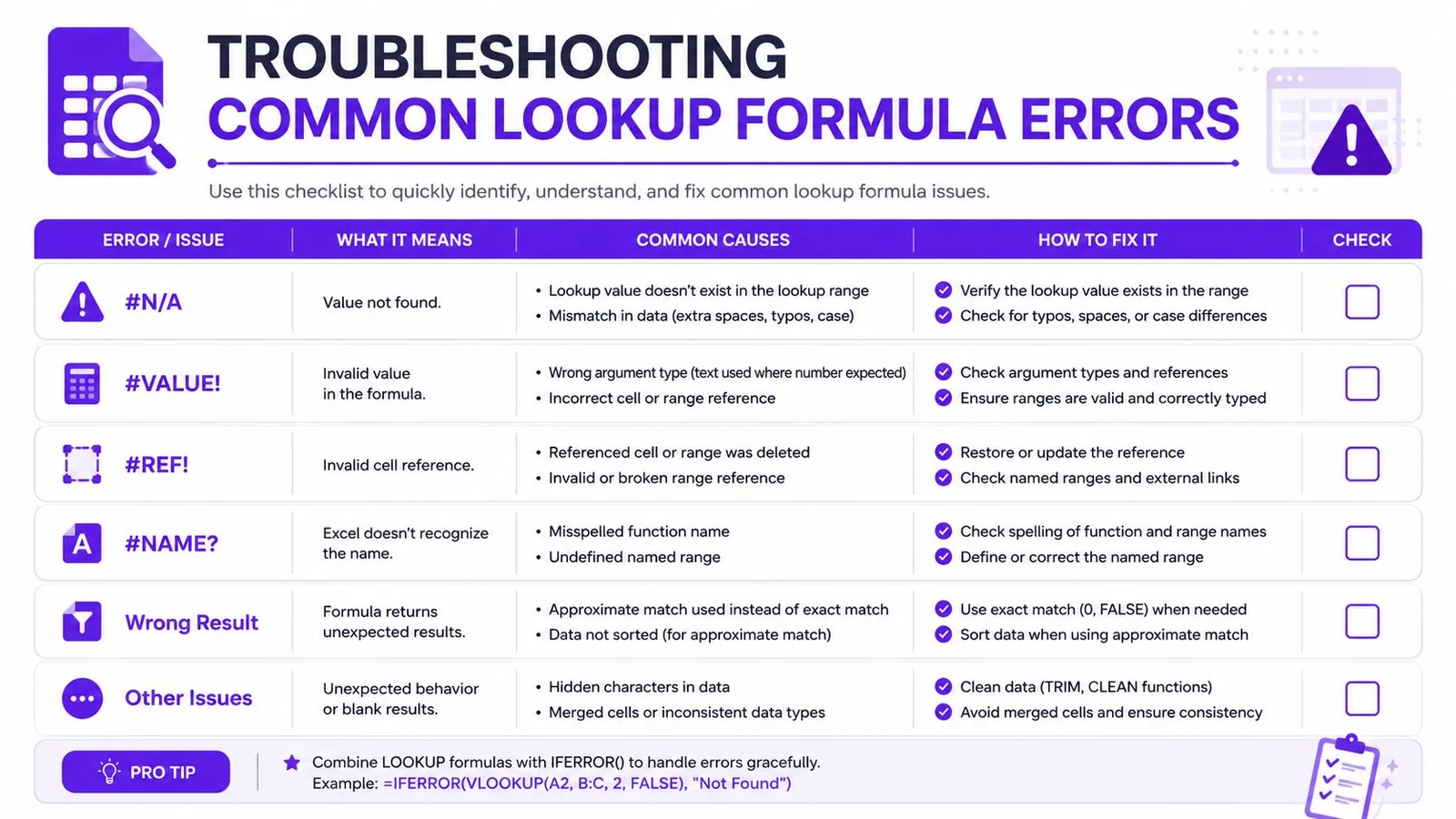
A practical cleanup workflow is to normalize types, trim spaces, and test the lookup key in isolation before layering on nested logic. Once the data is stable, the formula usually gets much simpler. When the data isn’t stable, the best lookup function in the world will still return the wrong row with perfect confidence.

See AI data cleaning for Google Sheets if your source tables keep arriving with inconsistent IDs, messy separators, or hidden formatting that keeps breaking exact matches.

Generating and Debugging Lookup Formulas with GPT Workspace

Complex lookup formulas are easy to mistype and annoying to debug by hand, especially when you’re juggling cross-sheet references, multi-criteria logic, or array output. GPT Workspace brings formula generation and debugging into Sheets with =GPT functions, so you can describe the lookup in plain language and get a formula back inside the workbook. It also supports selected-range analysis, which helps when you want the structure of the table inspected before choosing a function.

That matters because many lookup errors aren’t syntax errors at all. They’re design errors. You picked VLOOKUP for a layout that really needed XLOOKUP, or you copied an Excel pattern into Sheets without adjusting for array behavior.

A practical use pattern

• Generate a starting formula: Ask for a VLOOKUP, XLOOKUP, or INDEX/MATCH formula based on the columns in your sheet.
• Explain a broken formula: Paste the formula and ask why it returns #N/A or the wrong row.
• Convert the pattern: Turn a legacy lookup into a cleaner XLOOKUP version when the workbook allows it.

The value here isn’t magic. It’s speed and consistency. When the spreadsheet is large and the lookup logic is layered, a formula assistant can save a lot of trial and error, especially for teams that don’t want to memorize every function variation.

GPT Workspace formula generator for Sheets is one option for that workflow, and it fits best when you want help drafting or explaining formulas without leaving Google Sheets. For teams that live inside spreadsheets, that kind of in-sheet assistance can keep lookup logic closer to the data it’s meant to serve.

Quick Reference for All Google Sheets Lookup Functions

Use this as the fast decision layer when a sheet is already open and the formula needs to be right on the first try.

• VLOOKUP: =VLOOKUP(search_key, range, index, [is_sorted]). Best for simple vertical retrieval where the key is in the first column. Main limitation, it only searches left to right.
• XLOOKUP: searches a lookup range and returns from a separate result range. Best for exact-match work on new sheets. Main limitation, you still need to manage missing-value behavior explicitly.
• INDEX/MATCH: two-function pattern where MATCH finds position and INDEX returns the value. Best for flexible layouts and older workbooks. Main limitation, the formula is less compact than XLOOKUP.
• HLOOKUP: horizontal lookup across rows. Best for transposed or pivot-like tables. Main limitation, it only works naturally when the data runs across the top.
• LOOKUP: legacy sorted-range function. Best when the data is already sorted and simple. Main limitation, the sorted requirement makes it fragile.
• MATCH: returns position, not the value itself. Best for dynamic references and helper logic. Main limitation, it doesn’t retrieve data on its own.

If you’re choosing between XLOOKUP and VLOOKUP, start with the table shape and the error tolerance you need. If you’re stuck debugging a weird result, jump back to the troubleshooting section and check the data before the formula. If you’re working inside older sheets, INDEX/MATCH is still the most flexible fallback.

---

If your team keeps fighting broken lookup formulas, GPT Workspace can help generate, explain, and debug them directly inside Google Sheets with =GPT functions and range-aware analysis. Visit GPT Workspace to see how it fits into everyday lookup, cleanup, and analysis work inside Google Workspace.